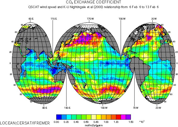
Determining CO2 exchange coefficients (K) from satellite wind speed
Several attempts have been made to relate air-sea gas transfer velocities, k, to wind speed, U. Relating k to U is not completely satisfactory because k is known to be driven by sea surface roughness which is not only dependent on wind speed and alternative approaches attempt to relate k to sea surface slopes (Frew et al., 2004) that is accessible using dual-frequency altimeters. However, scatterometer instruments provide a much better sampling than altimeters. Thence, in that study we choose to derive weekly 1° maps of K using satellite wind speeds.
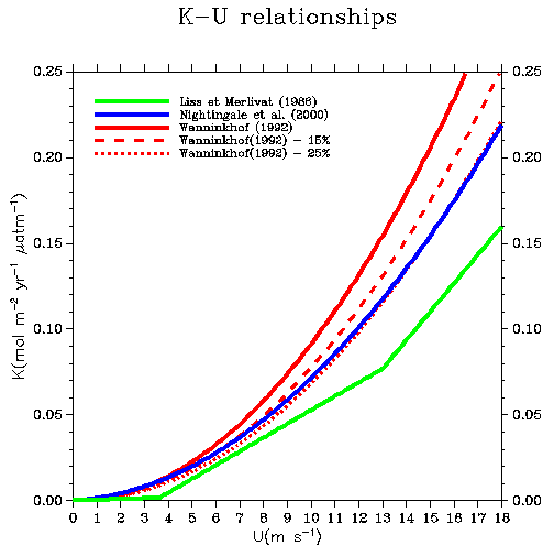
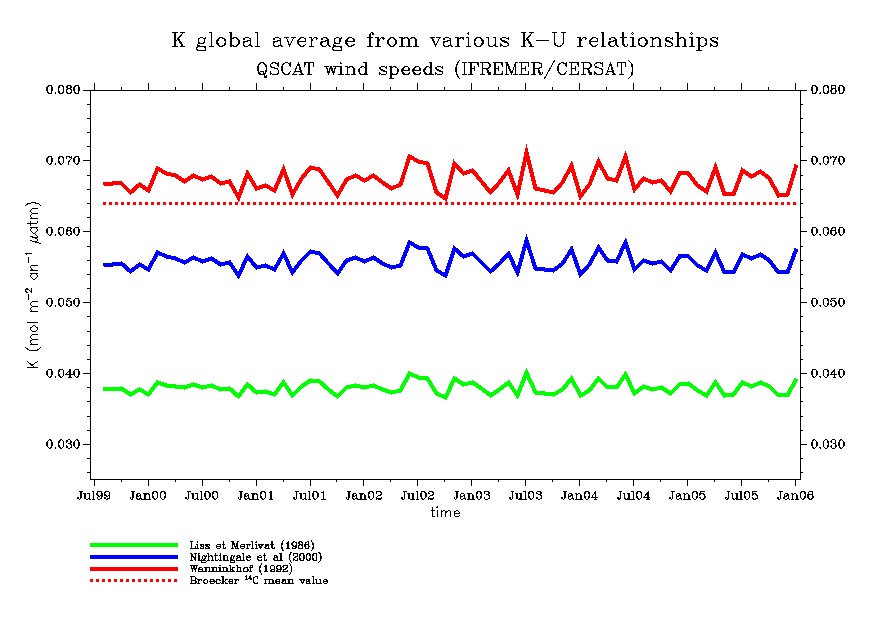
At present, three k-U relationships are commonly used to derive CO2 air-sea fluxes from wind speed and air-sea CO2 partial pressure gradient: Liss and Merlivat (1986), Wanninkhof (1992), Nightingale et al. (2000). This article describes the methodology used to map K from satellite wind speeds; we derive long term K global means from the three sets of CO2 exchange coefficients corresponding to the above k-U relationships and compare them with recent constraints derived from 14C revised inventories.