


Comparisons
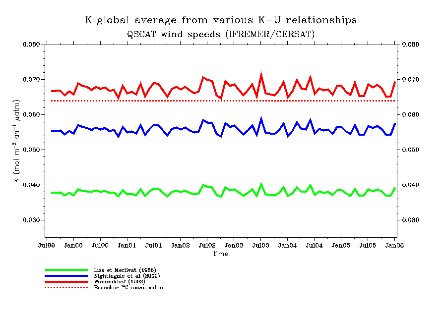 Global K weighted averages are deduced from monthly K maps from 1999 to 2006 as shown here. As expected from older studies, global mean K values deduced from these 3 k-U relationships are quite stable temporally (no seasonal cycle) but the K deduced from various relationships disagree by up to a factor 1.8 and this factor varies regionally (Boutin et al., 2002). Wanninkhof (1992) calibrated his k-U relationship on K deduced by Broecker et al., 1985 from Geosecs ocean 14C inventory: this corresponds to a mean K of 0.064 mol m-2 yr-1 matm-1 (Kbroecker); in addition Wanninkhof (1992) assumed a Rayleigh distribution of U with global mean U=7.4m/s. In fact, the QSCAT wind speed is on global average 7.8m/s (the discrepancy being possibly partly due to slight overestimate of QSCAT wind speeds) and does not exactly follow a Rayleigh distribution so that global Kw are on average 5% higher than the mean value assumed by Wanninkhof (1992) to calibrate his relationship.
Recently, new estimates of 14C ocean inventory have been proposed, either based on stratospheric modelling and/or analysis of WOCE data and/or reanalysis of Geosecs data:
- Hesshaimer et al. (1994) => Broecker Geosecs 14C inventory too high by 25%
- Peacock (2004) =>Revisited Geosecs inventory lower than Broecker by about 15%
- Naegler et al (2006) =>Revisited 14C inventory lower than Broecker by 12-20%
On global average, Kw, is 20% higher than the one derived with the Nightingale relationship, Kn; Kn are 15% lower than Kbroecker, in better agreement with Peacock (2004) and Naegler et al. (2005) new revisited inventory.